Yesterday I saw this retweet from @timelyportfolio that links to a gist by @gka.
The gist gave a few short scripts that can show you when your git commits take place during the day. I thought that was cool, so I took it a step (or five) further by writing it all up in R code and made nice wrapper functions for it and added interactive visualizations and made a shiny app… I just had a bit of fun. This is the result.
Note that all commit times are reported as PST timezone.
TL;DR: I’m dead before 10am — My prime working time is 2am — My supervisor Jenny Bryan has a very compatible schedule to mine — Hadley somehow learned in the past 3 years to be so productive that he doesn’t even work on weekends
This post shows a few plots and discusses them, but it can be more fun to play with the data yourself.
Table of contents
- Explore the data interactively yourself
- My work hours since first learning R
- My work hours in the past 6 months
- Adding marginal density plots to see exactly what times are alive/dead
- How’s my (ex) supervisor Jenny Bryan doing?
- And the grand finale: the R master Hadley
- Working on weekends
- R code used to generate this data
My work hours since first learning R
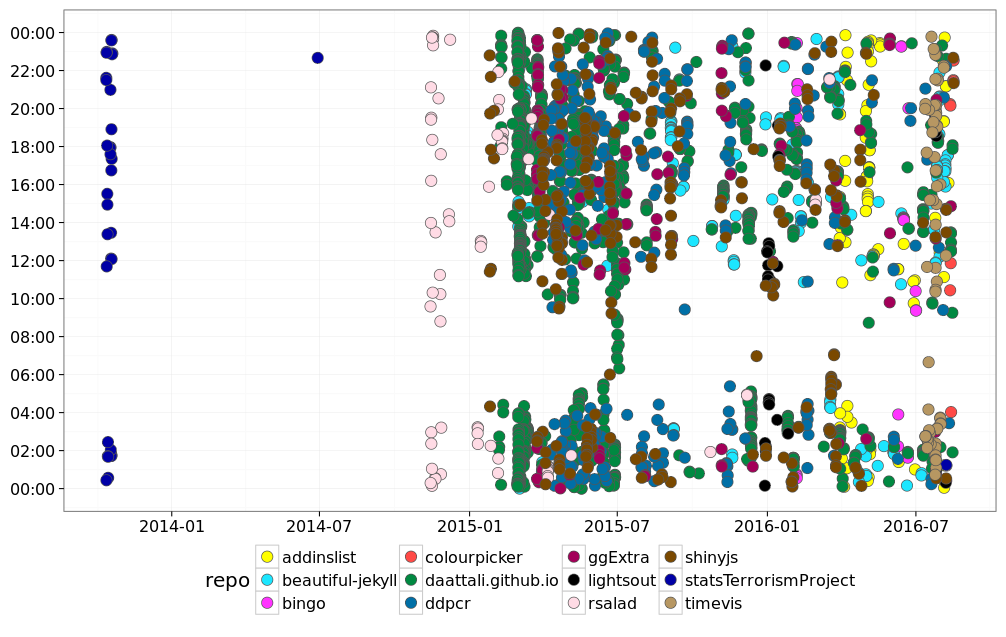
This plot shows the times of all my git commits since Sept 2013, colour-coded by git repo (aka project). If you go the app hosting this data, you’ll see this plot as fully interactive: you can zoom, move, or remove all observations from a specific repo by clicking on the repo name in the legend.
September 2013 is when I first learned R in the beginning of my masters degree, and the project I was working on then (statsTerrorismProject) was my final project for STAT545.
After taking my introductory R course, I spent the next year on my other masters courses and didn’t do any R-ing and coding, hence the giant gap. The next time I used git was when I took the second half of STAT545 in 2014, and that’s where I learned how to write a package – rsalad was my first R package, developed as homework. Then I didn’t do any open source work for a few months because I was working in a lab that wasn’t very supportive of that… And in January 2015 I started working with Jenny as my supervisor, and as you can see, I was pretty much busy with just about everything in the world except for my actual masters project! :)
A few things that are easy to notice:
- I refuse to work before 10am
- It looks like I work until 2am-4am fairly consistently
- I did a LOT of work on my website (dattali.github.io) around March 2015 (which is when I got the idea to make a website and when I released it)
- There were a few days in July 2015 where I started coding at 6am! Nope, that’s a lie, I was in Toronto that week so that’s actually 9am…
- It’s cool to see when I work on which projects. You can very clearly see the two-week effort on timevis in July 2016 for example
My work hours in the past 6 months
Observations
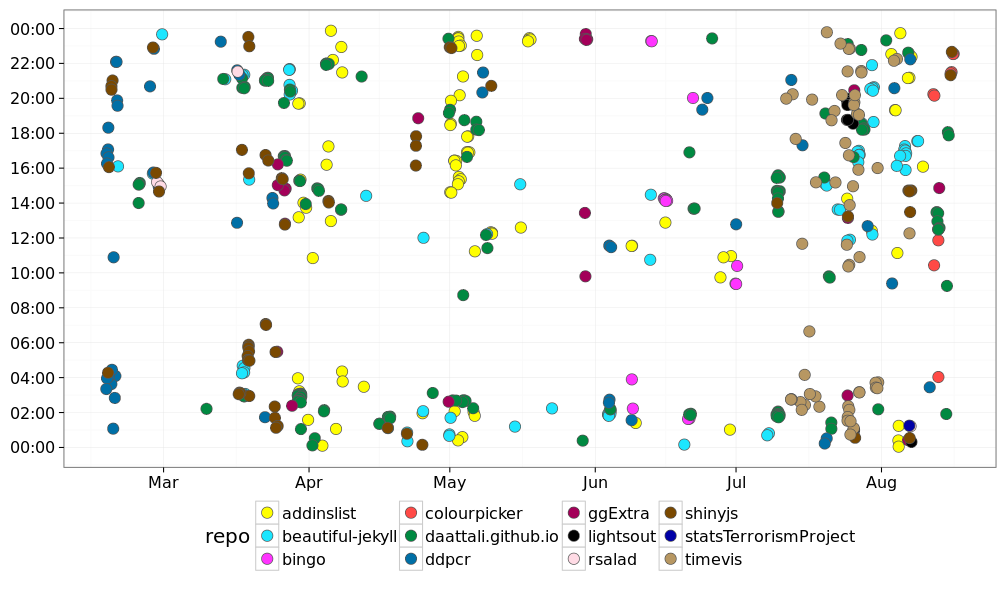
It’s interesting to see how my commits very closely relate to what’s going on in my life :)
- During Feb-March I was writing my masters thesis on my package ddpcr and you can see how I had one last burst of work on the package at the end of Feb, and then I completely stopped coding for a few weeks while I focused on writing. I was such a good boy.
- June seems like a dead month. I was in Toronto, Berkeley and Stanford for conferences and didn’t code at all. It’s cool how clearly that shows up!
- It’s nice to see that shinyjs has reached a fairly stable state and I don’t have to spend much time on it anymore
Adding marginal density plots to see exactly what times are alive/dead
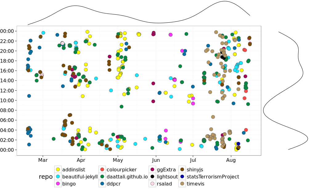
Just for fun, I can use my ggMarginal() function to add marginal density plots, to make it more clear when most of my commits take place.
How’s my (ex) supervisor Jenny Bryan doing?
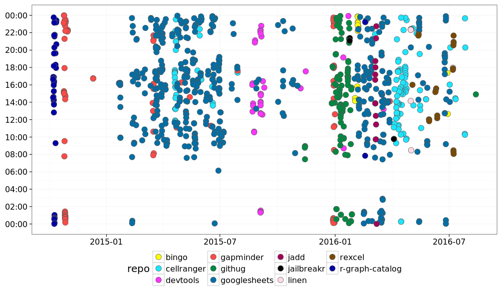
After working with Jenny for a couple years, I learned that we have very compatible schedules. It was very normal for us to exchange emails past midnight when we had a 9am class the following morning, and I’d often see her making commits at 1-2am when I was just getting in the zone!
With this graph we can see that our schedules really are very similar, although she is shifted 2 hours from me: I work 10am-4am, she works 8am-2am. What an early bird.
And the grand finale: the R master Hadley
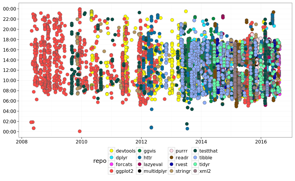
No introduction needed, the name speaks for itself. (Note these are all PST times)
Just one thing I’d like to note: we’ve all heard “this is going to be the year of ‘ggvis’!”, yet it looks like 2013 was the year-est of ‘ggvis’ so far :)
Working on weekends
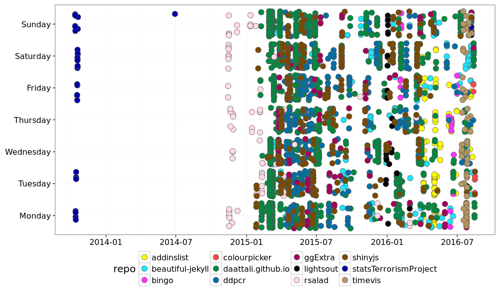
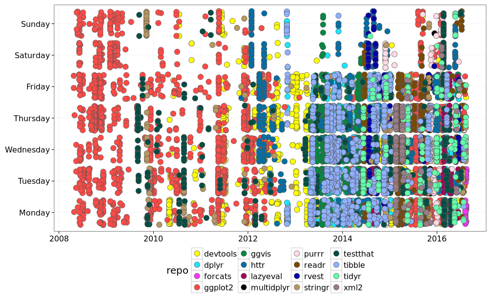
If you look at day of the week, you’ll see that weekends and weekdays are essentially the same to me.
But what’s amazing is that if you look at Hadley, he seems to be such a good time manager that he manages to almost never work on weekends in the past 3 years, despite producing output at a speed of a dozen adults. That discipline of not working on weekends is commendable.
R code used to generate this data
If you want to replicate these kinds of plots, here is the exact R code that was used to generate all the plots. The two functions you need to call are create_git_log_file() to generate the data file, and then plot_git_commits() to visualize the data.
I know this code isn’t amazing and could be optimized some more (I especially don’t love that I’m using system calls) but I wanted to get this out ASAP because I have real projects I need to work on :)
#' Plot the time or date of your git commits
#'
#' IMPORTANT: Before calling this function, you must use the `create_git_log_file()` function
#' to generate the data file that is used to make the plot!
#' You also need to have 'dplyr', 'git2r', 'ggplot2', 'ggExtra' and 'scales' packages installed.
#'
#' @param logfile The output from `create_git_log_file()`. This is a file containing all the
#'   necessary info for generating the activity plots. You must call `create_git_log_file()`
#'   first to create the data file, and then you can call this plot function to
#'   plot the data based on that file
#' @param num_months How many months back to look at your commits
#' @param plot_type What type of plot to output ("plotly", "ggplot", or "density")
#'   if you choose "density" then the result will be a ggplot2 plot with marginal density plots
#' @param x The variable to plot along the x axis (one of "repo", "time", "date", or "weekday")
#' @param y The variable to plot along the y axis (one of "repo", "time", "date", or "weekday")
plot_git_commits <- function(logfile, num_months = 6,
                             plot_type = c("plotly", "ggplot", "density"),
                             x = "date", y = "time") {
  if (!requireNamespace("dplyr", quietly = TRUE)) {
    stop("You need to install the 'dplyr' package", call. = FALSE)
  }
  if (!requireNamespace("ggplot2", quietly = TRUE)) {
    stop("You need to install the 'ggplot2' package", call. = FALSE)
  }
  if (!requireNamespace("scales", quietly = TRUE)) {
    stop("You need to install the 'scales' package", call. = FALSE)
  }
  if (!requireNamespace("ggExtra", quietly = TRUE)) {
    stop("You need to install the 'ggExtra' package", call. = FALSE)
  }

  plot_type <- match.arg(plot_type)

  if (!file.exists(logfile)) {
    stop("The git log file was not found", call. = FALSE)
  }

  if (!is.numeric(num_months) || num_months < 1) {
    stop("num_months must be a positive integer", call. = FALSE)
  }

  if (x == y || !all(c(x, y) %in% c("repo", "time", "date", "weekday"))) {
    stop('x and y must each be one of "repo", "time", "date" or "weekday" and must be unique', call. = FALSE)
  }

  # read the logfile and transform it into a useful dataframe
  gitdata <- get_git_df(logfile, num_months)

  # plot the result
  plot_git_commits_helper(gitdata, plot_type, x, y)
}

#' Create a data file with all the git commit info of a particular user for some repos
#'
#' In order to create this data file, all the git repos specified have to be cloned to your
#' local machine (this happens automatically). The result of this function is a data file with
#' information about git commits, and this file can be used as input for `plot_git_commit_time()`
#' (which will visualize the times of day commits were made)
#'
#' @param username The git name of the peson to track their commits (if you
#'   commit to git under multiple names, you can pass a vector of names)
#' @param repos A list of all the GitHub repos you want to analyze (all these
#'   repos will get cloned locally
#' @param dir The directory where all the git repos will
#' @param logfile THe name of the data file (the file with all the git lgs
create_git_log_file <- function(
  username = c("Dean Attali", "daattali"),
  repos = c("daattali/beautiful-jekyll",
            "daattali/shinyjs",
            "daattali/timevis",
            "jennybc/bingo"),
  dir ="git_repos_vis",
  logfile = "project-logs.csv") {

  if (!requireNamespace("git2r", quietly = TRUE)) {
    stop("You need to install the 'git2r' package", call. = FALSE)
  }

  if (!dir.exists(dir)) {
    dir.create(dir, recursive = TRUE, showWarnings = FALSE)
  }

  dir <- normalizePath(dir)

  # clone all the git repos into one folder and get their commit messages
  logs <- lapply(repos, function(repo) {
    # get the unique repo
    if (!grepl("/", repo)) {
      stop(repo, " is not a valid repo name (you forgot to specify the user)", call. = FALSE)
    }
    repo_name <- sub(".*/(.*)", replacement = "\\1", repo)
    repo_dir <- file.path(dir, repo_name)

    # clone the repo
    if (dir.exists(repo_dir)) {
      message("Note: Not cloning ", repo, " because a folder with that name already exists")
    } else {
      message("Cloning ", repo)
      repo_url <- paste0("https://github.com/", repo)
      git2r::clone(url = repo_url, local_path = repo_dir,
                   progress = FALSE)
    }

    # get the git log
    repo <- git2r::repository(repo_dir)
    commits <- git2r::commits(repo)

    dates <- unlist(lapply(commits, function(commit) {
      if (commit@author@name %in% username) {
        as.character(as.POSIXlt(commit@author@when@time, origin = "1970-01-01"))
      } else {
        NULL
      }
    }))
    data.frame(project = rep(repo_name, length(dates)),
               timestamp = dates,
               stringsAsFactors = FALSE)
  })

  # write the logs to a file
  logs <- do.call(rbind, logs)
  logfile <- file.path(dir, logfile)
  write.csv(logs, logfile, quote = FALSE, row.names = FALSE)

  if (file.exists(logfile)) {
    message("Created logfile at ", normalizePath(logfile))
  } else {
    stop("The git log file could not get creatd for some reason", call. = FALSE)
  }

  return(logfile)
}

#--- Helper functions ---#

get_git_df <- function(logfile, num_months) {
  library(dplyr)

  date_cutoff <- as.POSIXct(seq(Sys.Date(), length = 2, by = paste0(-num_months, " months"))[2])
  gitdata <- read.csv(logfile, stringsAsFactors = FALSE) %>%
    dplyr::filter(project != "") %>%
    dplyr::mutate(ts = as.POSIXct(timestamp)) %>%
    dplyr::filter(ts >= date_cutoff) %>%
    dplyr::mutate(
      repo = as.factor(project),
      date = as.Date(ts),
      time_short = strftime(ts, format = "%H:%M"),
      time = as.POSIXct(time_short, format = "%H:%M", tz = "UTC"),
      weekday = factor(weekdays(date),
                       levels = c("Monday", "Tuesday", "Wednesday",
                                  "Thursday", "Friday", "Saturday", "Sunday"))
    ) %>%
    dplyr::select(repo, date, time_short, time, weekday) %>%
    droplevels()
  gitdata
}

plot_git_commits_helper <- function(gitdata, plot_type = "plotly", x = "repo", y = "time") {
  # Define a large set of distinct colours
  all_cols <- c(
    "#FFFF00", "#1CE6FF", "#FF34FF", "#FF4A46", "#008941", "#006FA6", "#A30059", "#000000",
    "#FFDBE5", "#7A4900", "#0000A6", "#B79762", "#004D43", "#8FB0FF", "#63FFAC", "#997D87",
    "#5A0007", "#809693", "#FEFFE6", "#1B4400", "#4FC601", "#3B5DFF", "#4A3B53", "#FF2F80",
    "#61615A", "#BA0900", "#6B7900", "#00C2A0", "#FFAA92", "#FF90C9", "#B903AA", "#D16100",
    "#DDEFFF", "#000035", "#7B4F4B", "#A1C299", "#300018", "#0AA6D8", "#013349", "#00846F",
    "#372101", "#FFB500", "#C2FFED", "#A079BF", "#CC0744", "#C0B9B2", "#C2FF99", "#001E09",
    "#00489C", "#6F0062", "#0CBD66", "#EEC3FF", "#456D75", "#B77B68", "#7A87A1", "#788D66",
    "#885578", "#FAD09F", "#FF8A9A", "#D157A0", "#BEC459", "#456648", "#0086ED", "#886F4C",
    "#34362D", "#B4A8BD", "#00A6AA", "#452C2C", "#636375", "#A3C8C9", "#FF913F", "#938A81",
    "#575329", "#00FECF", "#B05B6F", "#8CD0FF", "#3B9700", "#04F757", "#C8A1A1", "#1E6E00",
    "#7900D7", "#A77500", "#6367A9", "#A05837", "#6B002C", "#772600", "#D790FF", "#9B9700",
    "#549E79", "#FFF69F", "#201625", "#72418F", "#BC23FF", "#99ADC0", "#3A2465", "#922329",
    "#5B4534", "#FDE8DC", "#404E55", "#0089A3", "#CB7E98", "#A4E804", "#324E72", "#6A3A4C")

  library(ggplot2)

  p <- ggplot(gitdata, aes_string(x, y, label = "time_short")) +
    geom_point(aes(fill = repo), col = "#555555", size = 5,
               shape = 21, position = position_jitter()) +
    theme_bw(20) +
    xlab(NULL) + ylab(NULL) +
    scale_fill_manual(values = all_cols[seq_along(unique(gitdata$repo))]) +
    theme(legend.position = "bottom")

  if (x == "date") {
    p <- p +
      scale_x_date()
  } else if (x == "time") {
    p <- p +
      scale_x_datetime(labels = scales::date_format("%H:00"), date_breaks = "2 hour")
  } else {
    p <- p + ggExtra::rotateTextX()
  }

  if (y == "date") {
    p <- p +
      scale_y_date()
  } else if (y == "time") {
    p <- p +
      scale_y_datetime(labels = scales::date_format("%H:00"), date_breaks = "2 hour")
  }

  if (plot_type == "plotly") {
    if (!requireNamespace("plotly", quietly = TRUE)) {
      stop("You need to install the 'plotly' package", call. = FALSE)
    }
    if (x == "time") {
      tooltip <- c("fill", "label", "y")
    } else if (y == "time") {
      tooltip <- c("fill", "x", "label")
    } else {
      tooltip <- c("fill", "x", "y")
    }

    p <- plotly::ggplotly(p, tooltip = tooltip)
  } else if (plot_type == "density") {
    p <- ggExtra::ggMarginal(p)
  }

  p
}
